This project has received funding from the European Union’s Horizon 2020 research and innovation programme under grant agreement No 766186. 
Thiago Rios
What a rollercoaster! A lot happened in the past three years of ECOLE and I am happy to see how far we got and how much nice work we have done. Participating in the project was a great opportunity to fast-track the start my career in research within an industrial scenario. Even though the pandemic caused some change of plans, I think we found nice ways to cope with the challenges and still have our workshops and collaborate with each other. The conferences, workshops, and other events that I took part during the project were very important to strength my technical and soft skills, as well as they allowed me to expand my personal and professional network. Now I am going through the last steps of finishing my PhD thesis and already looking forward for facing new challenges in my career as a researcher.
Sneha Saha
For the past 3.5 years, I have been working as an early-stage researcher in the ECOLE project, where my research focused primarily on the field of application of deep learning and machine learning techniques to real-world applications. Currently, I am in the final stage of my PhD and now writing my thesis. Doing applied research in the industry (HRI-EU) helped me to understand how design optimization is performed in an industrial scenario and I supported them in the implementation of machine learning and optimization techniques to solve such problems. Also, during the project, I got guidance from the university for conducting our research, and I had the chance to constantly collaborate with another ESR on conference papers and reports, which helped me to gather expertise from different domains. Lastly, the training offered by ECOLE helped me to enhance discipline-related and soft skills, as well as to expand our professional network.
Sibghat Ullah
I joined the ECOLE project in November 2018 after finishing my Masters in Data Science. For me, the journey of becoming an independent researcher in the field of Artificial Intelligence started with ECOLE. During my time as an early-stage researcher, I learned and improved my technical as well as interpersonal skills. Moreover, I improved my broader understanding about Artificial Intelligence and its role in our future. As James Burke states, “Scientists are the true driving force of civilization”. Analyzing this statement in this digital era of ours reveals the accomplishments that researchers involved in ECOLE have achieved. I am proud to have been part of an exciting journey, which involved working with lead scientists and enthusiastic young individuals. As a group member, I had a lot of fun and interaction with the other early-stage researchers and would like to work with them in future as well. Lastly, I would like to thank everyone behind the scenes who made the ECOLE project a reality. This includes the local researchers in each institution as well as the support and managerial staff involved. Thank You.
Duc Anh Nguyen
I started my PhD journey as a member of the ECOLE project in 2018 Oct. I had an excellent opportunity to work with world-leading researchers and young colleagues from HRI-EU, NEC-EU, Birmingham University, Leiden University, etc. Honestly, I learned a lot from this project in professional and soft skills. The knowledge and skills I equipped during the ECOLE project allow me to become an independent researcher in the field of data science and (automated) machine learning. Lastly, I would like to thank everyone who was involved in the ECOLE project; we had a great time working together.
Jiawen Kong
How time flies! Our ECOLE project is coming to an end, and I am also approaching my PhD graduation. During the past 3.5 years, I have always felt grateful for being a member of ECOLE. I must say that I have grown a lot, both in life and academically. Looking back, my interview with Thomas in Leiden was the first time that I travel alone. By now, I have travelled a lot by myself to attend conferences, training events and secondments. Back in 2018, I just graduated as a Master’s student in Statistics with only “book” knowledge. Now, I have finished my secondments in three industrial partners and equipped myself with state-of-the-art expertise in my research-related field, i.e. class imbalance learning. I would like to say “thank you” to all my supervisors; they not only supervise me in research but are considerate when I feel stressed and isolated during COVID-19. I also would like to show my respect to my colleagues in ECOLE; they are always creative, cooperative and friendly. I believe that the years I spent in ECOLE are one of the most valuable times in my 20’s.
Stephen Friess
It were crazy times. I stumbled upon the position as Early Stage Researcher first within summer 2018 through recommendation of a friend. Wanting to return to research, it was a welcome opportunity. Working daytime at a software company while putting together my interview presentation in the evening was stressful. But the work paid off. Having received the news of being accepted was crazy to me. But even more, the topics I was able to study within this period of time. From learning- and developmental biology inspired methods and the synergies between them in artificial intelligence, to design optimization within the automotive industry and novel machine learning methods for processing graph data. But more over the experiences lastingly shaped me by acquiring new and strengthening existing vital skills in being questioning, determined and assertive as a researcher as well as understanding the importance and quality of my own ideas. I therefore want to deeply thank my supervisors for supporting me on this journey and enabling this to become a possibility.
Gan Ruan
Time flies like an arrow. I was just feeling like our ECOLE project starts yesterday, but actually it ends soon. Recalling the moment when I received the offer sent from Dr Shuo Wang representing the ECOLE board, I was extremely happy to be exploded and felt I was the luckiest guy in the world, as this project provides me with a very precious opportunity to continue my research with the world-wide renowned Universities and Institutes as well as experienced scholars. Now, standing at the near-ending point of this project, I find that what I have experienced and learnt in this project have not disappointed me at all. Instead, it has beyond my original expectations a lot. In the past 3 and a half year, I have obtained fundamental knowledge via taking necessary courses arranged within the project, which I found is very beneficial to my later research. In addition, I also gain valuable experience of how to do meaningful research under the patient and kind supervision of ECOLE supervisors, which is extremely helpful to my future research life. Besides, through attending all kinds of activities, workshops, conferences and so on organized or funded by the ECOLE project, I have widen my horizon on my research and had a basic understanding on the research trend. At the same time, I have also gained experience and practiced my communication and presentation skills through communicating with peer and making public presentations. In addition to the research staff obtained within the project, I also made friend with other ESRs via attending above mentioned research activities and rest self-organized entertainment activities, tries to learn from each other to build up my own personality. Last but not least, I would like very thank for the understanding and supporting of the ECOLE board on my research and life in the period of my getting stuck in China due to the Covid.
Giuseppe Serra
It all started back in 2017, during my MSc thesis internship. At that time, I got a taste of what being a researcher means, and I liked everything about it. Consequently, after my MSc graduation, I was sure to continue my journey in the research field. After some applications, I was lucky enough to get accepted into the ECOLE project to start my doctorate. Now, taking a look back at the past three years, everything was much harder than I was expecting. Also, due to very well-known reasons, we missed many opportunities that are the essence of being a PhD student. Nonetheless, it was an incredible experience. Every small chat, discussion, meeting, or presentation, even remotely, with supervisors, scientists, and PhD fellows was a step towards improving me as a researcher, but also as a person. I learned a lot from each piece of advice, each comment I got, and from each challenge I encountered during this period. Words could never be enough, but I am thankful for the opportunity given and I believe that, with this wealth of experience, I will still learn a lot in the future to try to become as good as the supervisors that accompanied us during this journey.
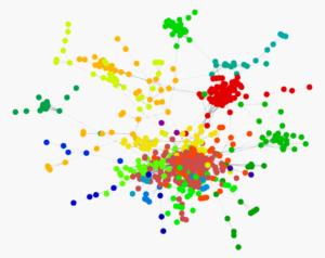
Figure 1. Visualization of a social network dataset of Facebook pages with mutual likes [1]. Different colours indicate different communities in the social network.
In the real world, a variety of data stemming from different application domains such as social networks, molecular chemistry, recommender systems and natural language processing [2] is best represented in the form of graphs. Meaning, particularly as pairs of adjacency matrices A, which represent the graph structure, and feature matrices X, which represent the contents of the graph elements.
For N nodes and C features, the adjacency matrix A is of size NxN, i.e. every pair of nodes has an entry Aij, and the feature matrix X is of size NxC, i.e. every node is represented by row vector of C features. The adjacency matrix essentially represents the connections between nodes in a graph. If two nodes i and j are connected, the respective element in the adjacency matrix is Aij = 1, otherwise Aij = 0.
Unfortunately, most of the traditional learning algorithms are unable to adequately account for the highly irregular and non-Euclidean structure of graphs. Thus, we require specialized architectures to process them. In the following, we will therefore provide an introduction to recently developed techniques for graph neural networks (GNN) [2, 3] which have been defined in analogy to traditional operations.
Graph Convolution Layers
While a variety of methods [3, 4] have been developed within the recent years as convolution operations, a very popular one is the one developed by Kipf & Welling [5]. Specifically, they consider graph convolutions as defined by
![]()
with a trainable weight matrix W(n) of size CxF with F filters, further H(0)=X the input feature matrix and the adjacency matrix Â=A+I with self-connections, as well as the degree matrix Dii = Σj Dij . The first four multiplicative terms can be interpreted as an aggregation operation over all features of the neighbors of a node. Thus, for each node i in the feature matrix X, we average over all features in the immediate neighborhood of i. Intuitively, the application of the graph convolution layer can be interpreted as a calculation of node embeddings, i.e. representations of the graph nodes in a low-dimensional vector space. This can work comparably well even if the weight matrix W is just randomly initialized (e.g. Fig. 2) and we find that nodes roughly group according to their community.

Figure 2. Column 1: Node embedding retrieved using graph convolutional layers. Column 2 & 3: The aforementioned social network graph coarsened by two levels.
Graph Pooling Layers
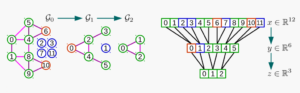
Figure 3. For a given input graph with 8 nodes which is supposed to be coarsened by 2 levels, the Graclus algorithm adds 4 additional feature-less fake nodes (left side). The resulting coarsened graphs can be rearranged into a balanced binary tree structure (right side), which can be pooled in analogy to 1d signals.
A variety of pooling layers have been likewise defined. One popular example is the one developed by Defferrard et al. (2016) [5] based upon the Graclus algorithm [7]. Pooling works largely in analogy to one 1D signals, however to do so, the Graclus algorithm conducts first in advance a graph coarsening step based upon calculating l levels of graph cuts of the original A adjacency matrix, such that
![]()
with coarsened adjacency matrices Aj* of size Nj* x Nj* , where j=0,…,l indicates the coarsening level and a permutation matrix P likewise of dimension Nj* x Nj*. Note, that the Graclus algorithm extends any given input graph with N nodes by adding Δ feature-less fake nodes, such that N* = N + Δ and further permuting the original node arrangement, such that the graph can be converted into a balanced binary tree. Thus, the original feature matrix must be converted by means of applying the permutation matrix P such that X*=PX. Based upon the permuted feature matrix, which is ordered according to a balanced binary tree, pooling operations are then simply conducted branch-wise in analogy to 1D signals with
![]()
Note that even though recent work [8] has been questioning the utility of pooling operations in graph neural networks, one may be inclined to use them nevertheless to keep the analogy to traditional architectures. This is a reasonable decision as there does not seem to be a clear consensus established upon this topic yet.
Spare me a last moment of your attention…
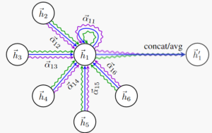
Figure 4. Illustration from [9] on how graph attention layers learn different weights for different node neighborhoods.
Research on graph neural networks is still a young and dynamic field and many of the presented techniques here might be either improved or completely neglected in the future. One interesting and promising new direction are for instance graph attention layers [9]. These heavily expand upon the previously presented technique of graph convolutions.
Now instead of averaging equally over all nodes in the neighborhood of a given node i, graph attention networks explicitly learn weights such that each node in the neighborhood is contributing differently. This comes much closer to how traditional convolution layers work for tensor data, but is particularly reflecting more recently developed attention mechanisms in neural networks.
In conclusion, research on graph neural networks is a young and dynamic field with exciting applications in a variety of domains. I hope this blog post could provide you a brief glimpse in some of the methods used in this new domain. 🙂
Note: All graphs in this article have been visualized with the NetworkX library [10].
References
[1] Rossi, R. and Ahmed, N., 2015, March. The network data repository with interactive graph analytics and visualization. In Proceedings of the AAAI Conference on Artificial Intelligence (Vol. 29, No. 1).
[2] Wu, Z., Pan, S., Chen, F., Long, G., Zhang, C. and Philip, S.Y., 2020. A comprehensive survey on graph neural networks. IEEE Transactions on Neural Networks and Learning Systems.
[3] Bronstein, M.M., Bruna, J., LeCun, Y., Szlam, A. and Vandergheynst, P., 2017. Geometric deep learning: going beyond euclidean data. IEEE Signal Processing Magazine, 34(4), pp.18-42.
[4] Niepert, M., Ahmed, M. and Kutzkov, K., 2016, June. Learning convolutional neural networks for graphs. In International conference on machine learning (pp. 2014-2023). PMLR.
[5] Kipf, T.N. and Welling, M., 2016. Semi-supervised classification with graph convolutional networks. arXiv preprint arXiv:1609.02907.
[6] Defferrard, M., Bresson, X. and Vandergheynst, P., 2016. Convolutional neural networks on graphs with fast localized spectral filtering. arXiv preprint arXiv:1606.09375.
[7] Dhillon, I.S., Guan, Y. and Kulis, B., 2007. Weighted graph cuts without eigenvectors a multilevel approach. IEEE Transactions on Pattern Analysis and Machine Intelligence, 29(11), pp.1944-1957.
[8] Mesquita, D., Souza, A.H. and Kaski, S., 2020. Rethinking pooling in graph neural networks. arXiv preprint arXiv:2010.11418.
[9] Veličković, P., Cucurull, G., Casanova, A., Romero, A., Lio, P. and Bengio, Y., 2017. Graph attention networks. arXiv preprint arXiv:1710.10903.
[10] Hagberg, A., Swart, P. and S Chult, D., 2008. Exploring network structure, dynamics, and function using NetworkX (No. LA-UR-08-05495; LA-UR-08-5495). Los Alamos National Lab.(LANL), Los Alamos, NM (United States).
Many effective sampling approaches have been developed in the imbalanced learning domain and the synthetic minority oversampling technique (SMOTE) is the most famous one among all. Currently, more than 90 SMOTE extensions have been published in scientific journals and conferences [1]. Most of the review papers and application work are based on the “classical” resampling techniques and do not take new resampling techniques into account. In this blog, we introduce three “new” oversampling approaches (RACOG, wRACOG, RWO-sampling) which consider the overall minority distribution.
The oversampling approaches can effectively increase the number of minority class samples and achieve a balanced training dataset for classifiers. However, the oversampling approaches introduced above heavily rely on local information of the minority class samples and do not take the overall distribution of the minority class into account. Hence, the global information of the minority samples cannot be guaranteed. In order to tackle this problem, Das et al. [2] proposed RACOG (RApidy COnverging Gibbs) and wRACOG (Wrapper-based RApidy COnverging Gibbs).
In these two algorithms, the n-dimensional probability distribution of minority class is optimally approximated by Chow-Liu’s dependence tree algorithm and the synthetic samples are generated from the approximated distribution using Gibbs sampling. The minority class data points are chosen to be the initial values to start the Gibbs sampler. Instead of running an “exhausting” long Markov chain, the two algorithms produce multiple relatively short Markov chains, each starting with a different minority class sample. RACOG selects the new minority samples from the Gibbs sampler using a predefined lag and this selection procedure does not take the usefulness of the generated samples into account. On the other hand, wRACOG considers the usefulness of the generated samples and selects those samples which have the highest probability of being misclassified by the existing learning model [2].
Inspired by the central limit theorem, Zhang et al. [3] proposed the random walk oversampling (RWO-Sampling) approach to generate the synthetic minority class samples which follow the same distribution as the original training data. Given an imbalanced dataset with multiple attributes, the mean and standard deviation for the ith attribute a_i (i ∈ 1,2,3,…,m) in minority class data can be calculated and denoted by μ and σ. Under the central limit theorem, as the number of the minority samples approaches infinite, the following formula holds
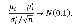
where μ’ and σ’ is the real mean and standard deviation for attribute a_i.
In order to add m synthetic examples to the n original minority examples, we first select at random m examples from the minority class and then for each of the selected examples x = (x_1, …, x_m) we generate its synthetic counterpart by replacing a_i(j) (the ith attribute in x_j, j ∈ 1,2,…,m) with µ_i – r_i * σ{i}/ sqrt{n}, where µ and σ denote the mean and the standard deviation of the ith feature restricted to the original minority class, and r_i is a random value drawn from the standard Gaussian distribution. We can repeat the above process until we reach the required amount of synthetic examples. Since the synthetic sample is achieved by randomly walking from one real sample, so this oversampling is called random walk oversampling.
[1] Fernández, A., García, S., Galar, M., Prati, R.C., Krawczyk, B. and Herrera, F., 2018. Learning from imbalanced data sets(pp. 1-377). Berlin: Springer.
[2] Das, B., Krishnan, N.C. and Cook, D.J., 2014. RACOG and wRACOG: Two probabilistic oversampling techniques. IEEE transactions on knowledge and data engineering, 27(1), pp.222-234.
[3] Zhang, H. and Li, M., 2014. RWO-Sampling: A random walk over-sampling approach to imbalanced data classification. Information Fusion, 20, pp.99-116.
Continuous optimization problems in real-world application domains, e.g., mechanics, engineering, economics and finance, can encompass some of the most complicated optimization setups. Principal obstacles in solving the optimization tasks in these areas involve multimodality, high dimensionality and unexpected drifts and changes in the optimization setup. Due to these obstacles and the black-box assumption on the optimization setup, traditional optimization schemes, e.g., gradient descent and Newton methods, are rendered inapplicable. The majority of the optimization schemes applied in these areas now focus on utilizing direct search methods, in particular Evolutionary Algorithms (EAs) and Surrogate-Assisted Optimization (SAO). In this blog, we provide a brief overview of our recently published paper [1] which focuses on high dimensional surrogate-assisted optimization.
SAO refers to solving the optimization problem with the help of a surrogate model, which replaces the actual function evaluations by the model prediction. The surrogate model approximates the true values of the objective function under consideration. This is generally done if the objective function is too complex and/or costly, and is therefore hard to optimize directly. The abstraction provided by the surrogate models is useful in a variety of situations. Firstly, it simplifies the task to a great extent in simulation-based modeling and optimization. Secondly, it provides the opportunity to evaluate the fitness function indirectly if the exact computation is intractable. In addition, surrogate models can provide practically useful insights, e.g., space visualization and comprehension. Despite these advantages, SAO faces many limitations in constraint handling, dynamic optimization, multi-objective optimization and high dimensional optimization.
Modeling high dimensional optimization problems with SAO is challenging due to two main reasons. Firstly, more training data is required to achieve a comparable level of modeling accuracy as the dimensionality increases. Secondly, training time complexity often increases rapidly w.r.t. both, the dimensionality and the number of training data points. Consequently, constructing the surrogate model becomes costlier.
Various methodologies have been proposed to deal with the issue of high dimensionality in SAO including divide-and-conquer, variable screening and mapping the data space to a lower dimensional space using dimensionality reduction techniques (DRTs). One of the most common DRTs is the Principal Component Analysis (PCA). PCA can be defined as the orthogonal projection of the data onto a lower dimensional linear space, known as the “principal subspace”, such that the variance of the projected data is maximized. Various generalized extensions of PCA have been established in the literature such as Kernel PCA, Probabilistic PCA and Bayesian PCA. On the other hand, Autoencoders (AEs) have been contemplated as feed-forward neural networks (FFNNs) trained to attempt to copy their input to their output, so as to learn the useful low dimensional encoding of the data. Like PCA, AEs have also been extended over the years by generalized frameworks such as Sparse Autoencoders, Denoising Autoencoders, Contractive Autoencoders and Variational Autoencoders (VAEs). Besides PCA and AEs, other important DRTs include Isomap, Locally-Linear Embedding, Laplacian Eigenmaps, Curvilinear component analysis and t-distributed stochastic neighbor embedding.
In this blog, we present some of the most important details from our paper [1], which empirically evaluates and compares four of the most important DRTs for efficiently constructing the low dimensional surrogate models (LDSMs). The DRTs discussed in our paper were PCA, KPCA, AEs and VAEs respectively. The comparison was made on the basis of the quality assessment of the corresponding LDSMs on a diverse range of test cases. There were a total of 720 test cases based on the combinations of ten test functions, four DRTs, two surrogate modeling techniques and three distinct values for dimensionality and latent dimensionality each. Furthermore, the quality assessment of the LDSMs was based on two criteria: modeling accuracy and global optimality. Based on the results in our paper, we believe following conclusions could be drawn:
Although our paper provided a comprehensive analysis on the performance of the LDSMs based on the four DRTs, there are a few limitations to discuss. Firstly, the study focused on unconstrained, noiseless, single-objective optimization problems. Therefore, the results could not be generalized to more complex cases. Secondly, the study did not focus on the size of the training sample size which can be crucial in many cases. Based on these rationales, we believe that further work is necessary to validate these findings on more complex cases, e.g., multiple-objectives, optimization under uncertainty, constraint handling and real-world applications.
References
[1] Ullah, Sibghat, et al. “Exploring Dimensionality Reduction Techniques for Efficient Surrogate-Assisted Optimization.” 2020 IEEE Symposium Series on Computational Intelligence (SSCI). IEEE, 2020.
In this blog series, I am introducing python Hyperparameter Optimization (HPO) and HPO libraries. Before reading this post, I would highly advise that you read my previous post. In this blog, I would introduce the python version of SMAC [1-3] (Sequential Model-based Algorithm Configuration), so-called SMAC3. SMAC is a Bayesian optimization’s variant, a well-known tool for hyperparameter optimization. It was first introduced in java (can be found here). Over years of development, SMAC is widely used in the machine learning community. There are even several well-known automated machine learning (AutoML) frameworks built on top of SMAC, such as auto-weka [4], auto-sklearn [5]. In general, SMAC has several facades designed for these different use cases, e.g. SMAC4AC, SMAC4HPO, SMAC4BO, the detailed information on these facades can be found here .
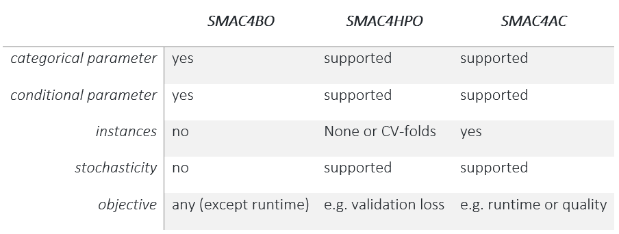
In this work, we introduce SMAC4HPO (without instances) and use the same example as my previous posts. Other usages of SMAC will be introduced in my future posts. In practice, to use SMAC, we will need three parts:
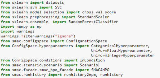
Figure 1. Import the necessary libraries.
Besides common type of hyperparameters such as Continuous, Nominal, and Ordinal hyperparameters; SMAC also supports Forbidden, conditional parameters.

Figure 2. The Hyperparameter search space includes two supervised machines learning: Support Vector Machine (SVM) and Random forest (RF).
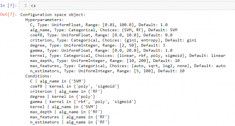
Figure 3 An example of SMAC’s Search space object.
The objective function in this blog is the same in my previous blog.
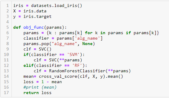
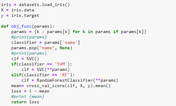
Figure 4. The objective function, use the classic Iris data set and do two supervised machines learning: Support Vector Machine (SVM) and Random forest (RF).
In the last step, we can config the optimizer SMAC by a scenario’s object.
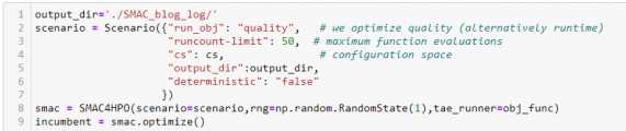
Figure 5. Tuning scenario.
Finally, SMAC will reports the best configuration. The detailed tuning process is stored in output_dir folder which we defined in the previous step. Note, this tuning historical can be restored and (possible) to continues the tuning process.
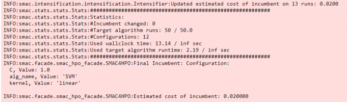
Figure 6. An example of SMAC’s result.
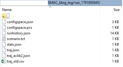
Figure 7. SMAC’s Output folder.
The code for this article is available in a JUPYTER NOTEBOOK ON GITHUB.
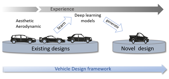
Artificial intelligence (AI) needs no introduction and it is already applied in diverse fields of research. Through the recent advances in AI, a current major trend is to collect and utilize existing digital design and simulation data for the application of data analytics and machine learning. Both help to increase the knowledge on the problem domain, provide a fast exploration of potential design ideas. The finding based on data analytics and machine learning may be communicated to the designer through an interactive design tool that would favor a cooperative character with well-thought interactions for proper guidance. Researches are already exploring the idea of “design suggestions” through AI interactive tools. Currently, there are several pieces of research on using AI for assistance in the design process, especially for 2D images. For example, AI-generated list of designs for presentations, i.e., a graphic designer could then select the font and size combination they find most useful (DesignScape). Other systems that have been proposed recently on 2D design level to provide real-time guidance to human users while drawing online — ShadowDraw [1] and SketchRNN [2]. Shadow relies on a database of images and provides feedback to user sketches by offering opaque visual layers of potentially similar objects. SketchRNN [2] is a generative, deep neural network trained on a database of drawing sequences by human users. When presented with a novel sketch sequence for a pre-selected object class, the network proposes alternatives of next drawing steps to illustrate potential design directions. But in our research, we focus on a 3D design for the automotive domain. Our aim is to generate an automotive design assistive system to assist the designer through an interactive vehicle design tool that would favor a cooperative character with well-thought interactions for proper guidance [3] such that the human designers’ capabilities are enhanced rather than replaced [4].
Current engineering design development processes are enriched by a manifold of computer-aided design (CAD) and engineering (CAE) tools for various tasks. Like in many other fields, in the automotive industry a huge amount of digital data emerges from computational models that are processed for quantifying various vehicle characteristics according to the required fidelities of detail. As examples, complete car designs are simulated for aerodynamic drag efficiency, or finite element models of structural components are computed for stiffness or crash safety. Besides technical performance, successful and innovative designs naturally build upon further qualities such as aesthetic appeal, which typically relies on a human in the loop to ideate and realize envisioned conceptual design directions.
State-of-the-art AI methods offer a promising approach to the realization of such a cooperative design system (CDS), wherein particular generative models may be used to provide guidance or potential alternatives giving the designer the freedom to rethink, discuss, and adapt promising product directions. Essential to such an automotive CDS is a model that provides a representation of 3D geometries that allows to efficiently explore the design space and is able to generate novel and realistic car shapes. In contrast to a manual design of the representation which would be potentially biased or limited by human heuristics, geometric deep-learning offers generative methods such as (variational) auto-encoders (V)AE [5] that learn low-dimensional representations of existing 3D shape data in an unsupervised fashion.
So, in our recent paper [6], we, therefore, use a point cloud based variational autoencoder (PC-VAE) that builds on the point cloud autoencoder originally proposed in [7], and extended in [8], which has been successfully evaluated for engineering applications. We further evaluate the generative capability of our PC-VAE by evaluating two central aspects: (1) the realism of the sampled shapes and (2) the capability of the model to generate diverse, novel shapes. For future research, we aim to use our generative PC-VAE for generating 3D shapes with more technical performances to evaluate a car design from aerodynamics or structural point of view. We will keep you updated about our work in our future blog post.
[1] Y. J. Lee, C. L. Zitnick, and M. F. Cohen, “ShadowDraw: real-time user guidance for freehand drawing,” in ACM Transactions on Graphics (TOG), vol.30, no. 4, Article 27, 2011.
[2] D. Ha and D. Eck, “A neural representation of sketch drawings,” in 6th International Conference on Learning Representations, ICLR 2018, Vancouver, BC, Canada, April 30 – May 3, 2018, Conference Track Proceedings, 2018.
[3] D. G. Ullman, “Toward the ideal mechanical engineering design support system,” Research in Engineering Design – Theory, Applications, and Concurrent Engineering, vol. 13, no. 2, pp. 55–64, 2002.
[4] J. Heer, “Agency plus automation: Designing artificial intelligence into interactive systems,” Proceedings of the National Academy of Sciences, vol. 116, no. 6, pp. 1844–1850, 2019.
[5] D. P. Kingma and M. Welling, “Auto-encoding variational bayes,” in 2nd International Conference on Learning Representations, ICLR, 2014, pp. 1–14.
[6] Sneha Saha, Stefan Menzel, Leandro Minku, Xin Yao, Bernhard Sendhoff and Patricia Wollstadt, “Quantifying The Generative Capabilities Of Variational Autoencoders For 3D Car Point Clouds”, in 2020 IEEE Symposium Series on Computational Intelligence (SSCI), Canberra, Australia, 1-4 December 2020 [Accepted].
[7] P. Achlioptas, O. Diamanti, I. Mitliagkas, and L. Guibas, “Learning representations and generative models for 3d point clouds,” 35th International Conference on Machine Learning, ICML, vol. 1, pp. 67–85, 2018.
[8] T. Rios, B. Sendhoff, S. Menzel, T. Back, and B. Van Stein, “On the Efficiency of a Point Cloud Autoencoder as a Geometric Representation for Shape Optimization,” in IEEE Symposium Series on Computational Intelligence, SSCI 2019, 2019, pp. 791–798.
Going through the PhD research feels very much like racing an endurance to me. We start fresh, with a nice pace and not completely sure about how it is going to end. Then, along the way, we learn how to manage resources, communicate to our team, and get around bumps and obstacles—even very big ones, such as the pandemic has been this year—to get to the end prepared for the next stage of our careers, with a nice work history and probably tired, but not burned out. We are heading now towards the end of our second year as PhD students, and here is a personal list with some of the lessons learned during this period of time.
#1 Making science is not all about the technique! Having a PhD research done requires a lot of technical work, regardless of the field of knowledge. However, communicating what we are doing is just as important and it might take some effort to communicate fluently to different audiences. Therefore, practicing is never too much, and participating in scientific seminars and discussions is important and can help us to improve our communication skills.
#2 Resilience from start to finish. Research is about pushing the science frontier beyond, which can be as tough as fascinating and joyful. Experiments do not always work out as expected and it can derail our publication plans, but that is just part of the journey. Hence, during the research we have to learn how to cope with problems that catch us by surprise and to literally science our way out of them. There is also no shame in asking for help! Discussing with friends, colleagues and supervisors about the research (including expectations) is healthy and helps us to keep the motivation throughout the PhD.
#3 Enjoy the opportunities! The PhD work is usually somewhere around that sweet spot between academic and corporate life. In the innovative training networks (ITNs), such as the ECOLE, we have plenty of chance to experience the work in the industry and academia, which have different dynamics and definitely helps us to think about where and how we would like to work in the future. Hence, if you have the chance to do internships or work outside the lab during the PhD, take it! It might push you out of the comfort zone, which is already hard to reach during the PhD, but it is a valuable experience.
#4 We have enough time to finish that, right? The answer might be “yes” but prefer to start sooner rather than later. Getting carried by the avalanche of tasks during the PhD is very easy, so being organized and thinking ahead of the deadlines is central, including for career plans. It helps us to foresee and thus avoid problems, allows us to think clearly on the structure of our manuscripts and to iterate our analyses more times before publishing them, improving the quality of our work.
These four points I took from my personal experience, but if you are interested in more tips or perspectives, many other PhD students already shared their experiences in [Nature](https://www.nature.com/collections/dhbegcaieb).
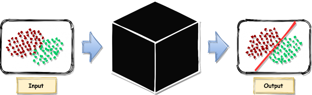
Thanks to their flexibility, applicability and effectiveness, machine learning (ML) models have become popular in many applications. Recently, deep learning approaches are reaching impressive performances on a variety of different tasks (e.g. computer vision, text classification) [1]. Despite good performances, there are still grey areas regarding these methods. Many works have proved how a deep learning method can be fooled by altering an image or a text with some perturbations. Experiments show that changes in an image would lead the model to classify it as something different (e.g. a tomato as a dog). Or that is possible to generate perturbed images that the model would classify with high confidence but are not recognizable by humans (e.g. a white noise as a tomato). In textual analysis, minimal perturbations in a document could lead to wrong topic classifications. Additionally, in many cases, the results are poorly explainable with the risk of creating and using decision systems that we do not understand. All these limitations raise reasonable concerns about the reliability of these models.
Depending on the application, we can identify different interpretability techniques for ML models [2]:
Feature relevance explanations: e.g. attention mechanism where a relevance score is computed to clarify which variables contribute to the final output.
The use of sophisticated machine learning models (considered as black-boxes), in industrial, medical and socio-economical applications is requiring a better understanding of the processes behind a final decision and of the decision itself [3]. The improper use of ML could lead to high-impact risks, especially if dealing with information that may be sensitive or decisions that may have a real impact. In medical application, how can we trust a diagnosis suggested by an algorithm with high accuracy but without a complete understanding of the output? In business decisions, how can a company make a profitable decision using ML without understanding if it is the right move or not? For all the above reasons, interpretability is getting more and more crucial across different scientific disciplines and industry sectors.
[1] Guidotti, R., Monreale, A., Ruggieri, S., Turini, F., Giannotti, F., & Pedreschi, D. (2018). A survey of methods for explaining black box models. ACM computing surveys (CSUR), 51(5), 1-42.
[2] Arrieta, A. B., Díaz-Rodríguez, N., Del Ser, J., Bennetot, A., Tabik, S., Barbado, A., … & Chatila, R. (2020). Explainable Artificial Intelligence (XAI): Concepts, taxonomies, opportunities and challenges toward responsible AI. Information Fusion, 58, 82-115.
[3] Lage, I., Chen, E., He, J., Narayanan, M., Kim, B., Gershman, S. and Doshi-Velez, F., 2019. An evaluation of the human-interpretability of explanation. arXiv preprint arXiv:1902.00006
Evolutionary multi-objective optimization has been leveraged to solve dynamic multi-objective optimization problems (DMOPs). DMOPs are characterized by multiple conflicting and time-varying objectives functions. Diversity maintenance and prediction methods are two mainstreams in solving DMOPs. It is impossible that any prediction methods can be very accurate in dynamic multi-objective optimization (DMO). Therefore, a hybrid diversity maintenance method [1] is to be investigated to improve the accuracy of prediction in DMO. This strategy is termed as DMS. More details of DMS can be found in [1].
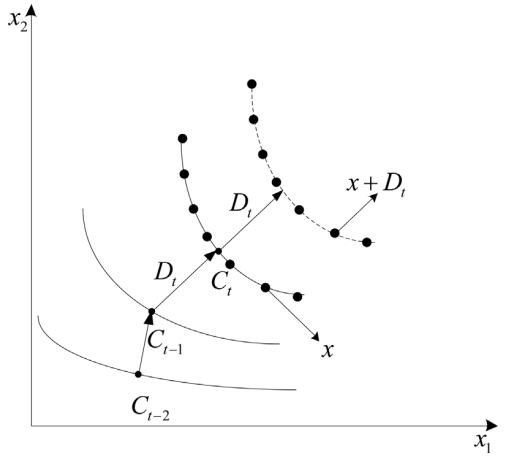
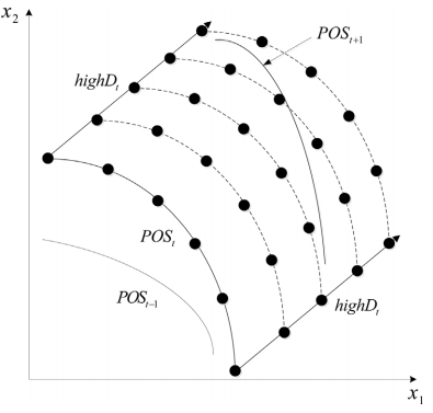
Due to the fact that changes in DMOPs always possess some regularity, it is intuitive to use prediction strategies to predict optimal solutions after changes. Therefore, loads of researches have been done regarding developing prediction strategies [2]. Here, a similar prediction strategy is applied. The prediction strategy makes use of the moving direction of centroid points of the past two time’s populations to predict the new location of Pareto optimal set (POS) [3]. The centroid of nondominated solutions is chosen as the centroid of a population. The prediction strategy is illustrated in Figure. 1. The solution set produced by this prediction is denoted as P_prediction.
The hybrid diversity maintenance method is to decrease the inaccuracy of the prediction as much as possible. It includes two strategies, gradual search strategy, and random diversity maintenance strategy.
Gradual search strategy
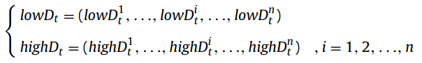
The gradual search strategy is used to find well-converged and well-distributed solutions around the predicted POS. This strategy makes use of the minimum point (low_t) and the maximum point (high_t) of non-dominated solutions in the population. The definition of the minimum point and the maximum point is defined in the following equation.
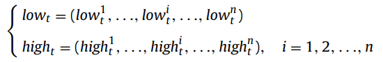
where n is the dimension of the decision space. Then the ith element of the minimum and the maximum point is defined as follows:
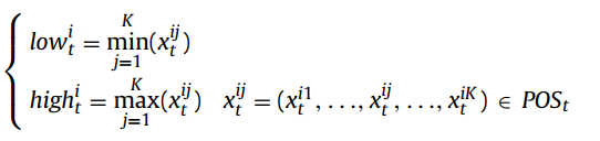
where K is the number of solutions in the nondominated solution set.
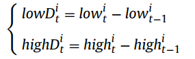
In this strategy, the moving direction is applied to determine the searching region. The moving directions of the minimum point and maximum point between two environmental changes are denoted by lowD_t and highD_t respectively.
where n is the dimension of the decision space. Then the ith element of the moving direction of the minimum point and maximum point referred to as lowD^i_t and highD^i_t is defined as:
Then the moving direction is selected by max(|lowD_t|, |highD_t|), |lowD_t| and |highD_t| are the length of the moving directions. Select the vector between these two moving directions with the larger length as highD_t. Lastly, generate N solutions through the following equation.
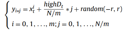
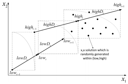
where r is a small radius. yi*j is the i * jth solution. x_t^i is the ith solution in the previous POS in the t_th environmental change. N is the number of individuals in the population. The detailed illustration of the gradual search is shown in Figure 2. The solution set produced by this gradual search strategy is denoted as P_GraSearch.
Random diversity maintenance strategy
The main idea of the random diversity maintenance strategy is to randomly produce solutions within the possible range of the next POS. The minimum and maximum points of the POS_{t+1} are firstly predicted by the following equation.
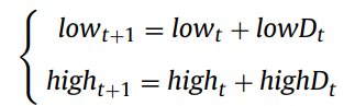
Then, solutions are generated through
where random(a, b) is a random function and returns a random value between a and b. The solution set produced by this random diversity maintenance strategy is denoted as PDM.
After generating those three solution sets, they are combined to select a nondominated solution set as the reinitialized population for the optimization.
In order to study the influence of the diversity maintenance on the prediction, the algorithm with prediction and the one with both prediction and diversity maintenance (DM) are used to run on several problems FDA1, DMOP2, F6, and F7 [1]. The mean IGD values are recorded during the optimization with 120 changes and plotted in Figure 4.
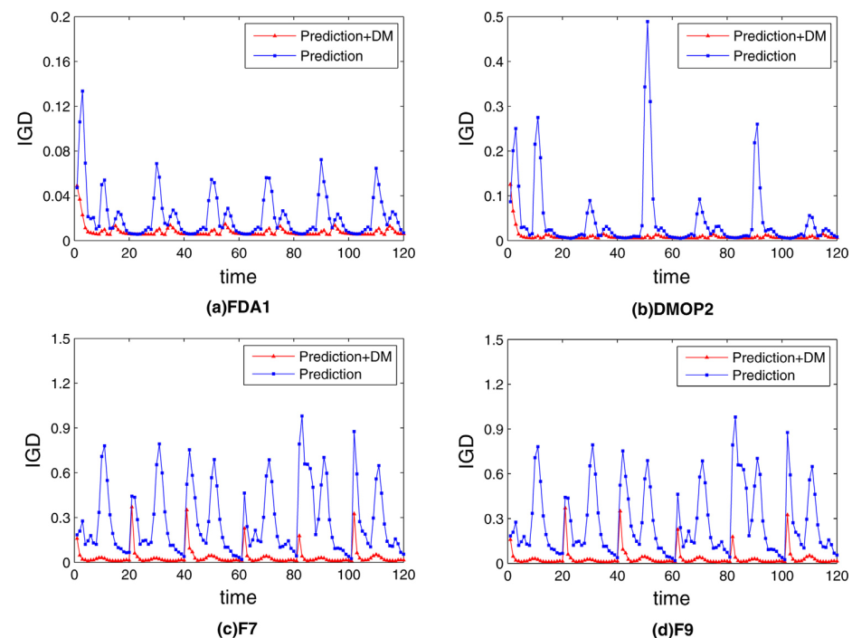
Figure 4. The average IGD over 20 runs versus time on (a) FDA1, (b) DMOP2, (c) F7 and (d) F9, DM represents the combined strategy with gradual search strategy and random diversity maintain strategy.
The algorithm with prediction and diversity maintenance strategies has better performance on convergence and distribution than that with the prediction alone. The diversity maintenance strategy gradually searches for more promising individuals, which prompts the convergence of the population and decreases the inaccuracy that the prediction may lead. Meanwhile, the diversity maintenance mechanism assists in the improvement of the diversity. Thus, DMS cannot only respond to both smooth and sudden environmental changes quickly and accurately but also perform well in later environmental changes. In other words, the results demonstrate that the diversity maintenance mechanism has a great promotion to the convergence and diversity in the optimization, and prediction has some influence on optimization to some extent.
[1]. G. Ruan, G. Yu, J. Zheng, J. Zou, and S. Yang, “The effect of diversity maintenance on prediction in dynamic multi-objective optimization,” Applied Soft Computing, vol. 58, pp. 631–647, 2017.
[2].Wu Y , Jin Y , Liu X . A directed search strategy for evolutionary dynamic multiobjective optimization[M]. Springer-Verlag, 2015.
[3]. M. Farina, K. Deb, P. Amato, Dynamic multiobjective optimization problems: test cases, approximations, and applications, IEEE Trans. Evolut. Comput. 8 (5) (2004) 425–442.
Most data-level approaches in the imbalanced learning domain aim to introduce more information to the original dataset by generating synthetic samples (check BLOG 3). However, in this blog, we introduce another way to gain additional information, by introducing additional attributes. We propose to introduce the outlier score and four types of samples (safe, borderline, rare, outlier) as additional attributes in order to gain more information on the data characteristics and improve the classification performance.
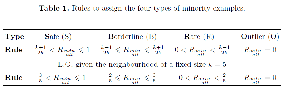
Napierala and Stefanowski proposed to analyze the local characteristics of minority examples by dividing them into four different types: safe, borderline, rare examples and outliers [1]. The identification of the type of an example can be done through modeling its k-neighborhood. Considering that many applications involve both nominal and continuous attributes, the HVDM metric is applied to calculate the distance between different examples. Given the number of neighbors k (odd), the label to a minority example can be assigned through the ratio of the number of its minority neighbors to the total number of neighbors (R_(min)/(all)) according to Table 1. The label for a majority example can be assigned in a similar way.
 Outlier Score
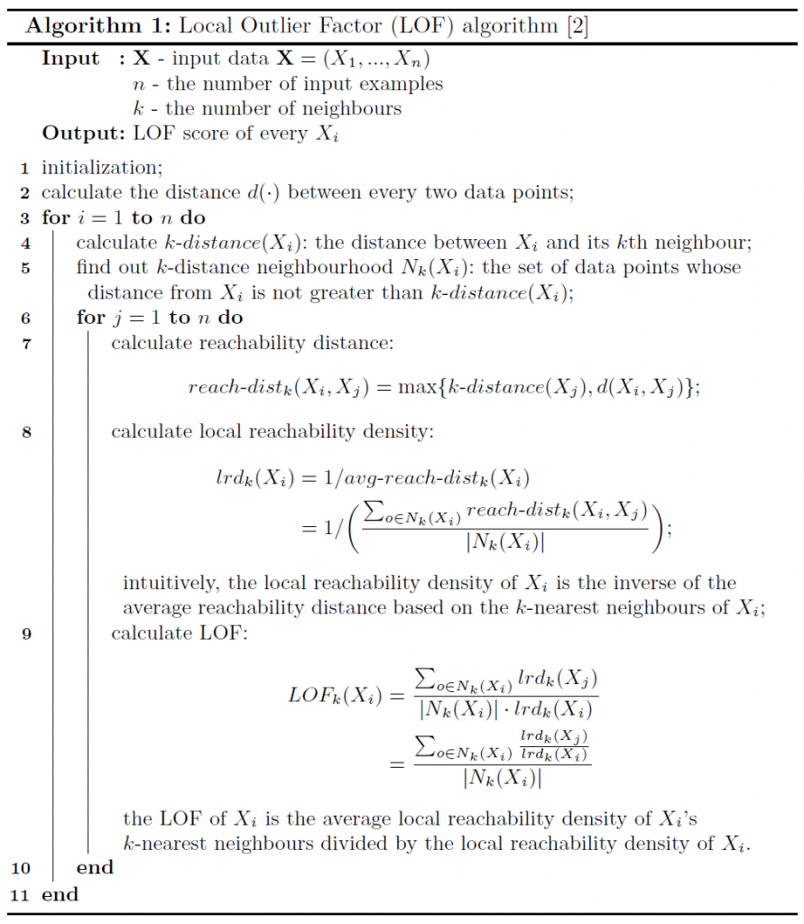
Many algorithms have been developed to deal with anomaly detection problems and the experiments in this paper are mainly performed with the nearest-neighbor based local outlier score (LOF). Local outlier factor (LOF), which indicates the degree of a sample being an outlier, was first introduced by Breunig et al. in 2000 [2]. The LOF of an object depends on its relative degree of isolation from its surrounding neighbors. Several definitions are needed to calculate the LOF and are summarized in the following Algorithm 1.
 Conclusions
According to our experimental results (can be checked here) [3], introducing additional attributes can improve the imbalanced classification performance in most cases (6 out of 7 datasets). Further study shows that this performance improvement is mainly contributed by a more accurate classification in the overlapping region of the two classes (majority and minority classes). The proposed idea of introducing additional attributes is simple to implement and can be combined with resampling techniques and other algorithmic-level approaches in the imbalanced learning domain.
[1]. Napierala, K. and Stefanowski, J., 2016. Types of minority class examples and their influence on learning classifiers from imbalanced data. Journal of Intelligent Information Systems, 46(3), pp.563-597.
[2]. Breunig, M.M., Kriegel, H.P., Ng, R.T. and Sander, J., 2000, May. LOF: identifying density-based local outliers. In Proceedings of the 2000 ACM SIGMOD international conference on Management of data (pp. 93-104).
[3]. Jiawen Kong, Wojtek Kowalczyk, Stefan Menzel and Thomas Bäck, “Improving Imbalanced Classification by Anomaly Detection” in Sixteenth International Conference on Parallel Problem Solving from Nature (PPSN), Leiden, The Netherlands, 5-9 September 2020 [Accepted]
In order to correctly apply Machine Learning for a given problem/data set, the practitioner has to set several free parameters, so-called “hyperparameters” such as the kernel function and gamma value in the Support Vector Machines. To select a good configuration of those hyperparameters which minimizes the loss value for a given data set, we need to do an external optimization process, which is known as hyperparameter tuning. There are many hyperparameter tuning approaches that have been introduced, e.g., Random Search, Grid Search, Evolution Strategies and Bayesian Optimization. For a simple problem with low dimensions of hyperparameter search space, we find the best configuration by trying many combinations of the input hyperparameters and choose the one with the lowest loss value. We could simply create a grid of hyperparameter values and try all of them, this method is named Grid Search; or randomly select some configuration, known as Random Search [1]. Grid Search is slow while random search is fast, but it is completely random, and we might miss the best configuration. However, both Grid Search and Random Search are easy to implement, thus, they are two of the most common methods. In this blog, we will introduce a smarter hyperparameter tuning method called “Bayesian Optimization” and one Pythonic implementation of Bayesian optimization, a framework named Hyperopt [5].
In practice, the search space is high dimensional and evaluating the objective function is expensive, thus, we want to try the promising configuration rather than try a random configuration from a grid uninformed by past trials. Luckily, Bayesian optimization can answer this question. Bayesian Optimization or Sequential Model-Based Optimization (SMBO)[2-4] is an approach based on history as it uses the historical information to form a surrogate probabilistic model of the objective function M = P(y|x), where x indicates candidate configuration and y indicates the probability of loss value on the objective function. Then, we choose the next candidate configuration by applying an Acquisition Function (e.g., Expected Improvement) to this surrogate model M. In summary, Bayesian Optimization differs from Grid Search and Random Search by keeping track of the evaluated results to concentrate on more promising candidate configuration.
To run this, we need three parts:
In this blog series, I will use the same example as my previous blog “MIP-EGO4ML: A python Hyperparameter optimisation library for machine learning”.
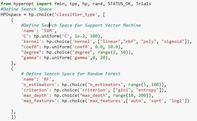
Figure 1. The objective function with the classic Iris data set and two supervised machines learning: Support Vector Machine (SVM) and Random forest (RF) respectively.
In the next step, we need to define a hyperparameter search space:
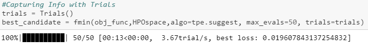
“Trials” is one special object, it records the return values by objective function for every single evaluation. However, Trial is an optional if we want to inspect the optimizing progression.
The code for this article is available in a JUPYTER NOTEBOOK ON GITHUB.
This article is a short introduction to Bayesian optimization and Hyperopt; as a blog in my hyperparameter optimization blog series. I will update more articles about hyperparameter optimization techniques in future posts. Apart from this article, I also published another article in this series:
MIP-EGO4ML: A python Hyperparameter optimisation library for machine learning
First of all, I pardon the delay. Today’s article was originally supposed to be about perspectives on knowledge transfer in intelligent systems, but the breadth and depth of this article were too much to be prepared in a firm and publishable form within just two weeks. Nevertheless, you can expect the article to be available in some form or another in the next months. So instead of today, I will give you a gentle introduction to the free-form deformation technique and introduce you to some tools for working with it.
 The free-form deformation technique was originally introduced by Sederberg & Parry in a paper published in 1986 at SIGGRAPH. Particularly, it introduces a technique to deform geometries by taking some loose inspiration from sculpturing. While there exist more modern techniques as of recently, the free-form deformation technique has the advantage that it is particularly fast and elegant to implement. We first start by parametrizing a control volume of the shape we want to deform by means of defining a set of three basis vectors S, T and U:
![]()
For a given point X in the control volume, the coefficients s, t & u can be calculated in the new basis using the equations:
![]()
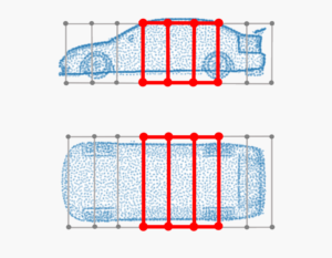
Note that the basis does not necessarily need to be orthogonal, thus we use the cross product. To define so called “control points“ to deform the geometry, we first start by defining a grid with l+1, m+1 and n+1 planes. Control points for the indices then lie at the intersections of the planes parametrized by i=0…l, j=0…m and k=0…m, such that Pijk :
![]()
Deformations Pijk of the shape can then be introduced by calculating the trivariate vector-valued Bernstein polynomial:

So far, just some very simple algebra. How do we get from these now to transformed cars?
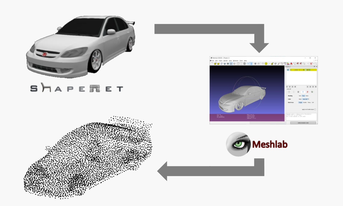 So we now have a basic understanding of the free-form deformation technique. How do we get from these basic deformation equations to transformed car shapes? First of all, we need some suitable models. For this reason, ShapeNet, a collaboration between researchers from Princeton, Stanford and a Chicago-based research institute, have made available a collection of over 50,000 different models online. While not primarily intended for the use in design optimization, the common frameworks in which geometric data is represented make them nevertheless suitable for any purpose one would like to consider. Just browse through their Taxonomy Viewer and you will pretty much find anything from late 70s SciFi spacecraft to consumer class cars from a well-known car manufacturer. Cool – so now we can get any model we would like. How do we apply free-form deformation to these now? Well, one solution would be to simply use NumPy-STL. STL (Standard Triangle Language) is a file format for CAD data. NumPy-STL was specifically designed to work with these files in a Python environment. Just drop in your Jupyter notebook or your command-line interface ‘pip install NumPy-stl’ and as soon as it is installed drop these few lines of code to load the STL file into a NumPy array of polygons:
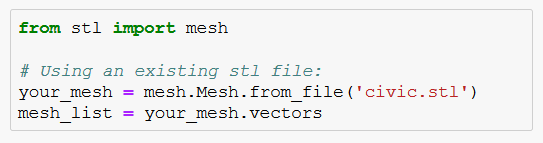 Technically, you are done now. The mesh_list is nothing else than a list of polygons, meaning in our case interconnected triangle surfaces which are sticked together to form the shape we want to work with. The triangles are each parametrized by three vectors pointing towards their corners. Thus, by modifying these vectors you change the size and orientation of the triangle and thus the shape of the car. In principle, we could stop with the blog article now, as you are now familiar with all the tools required to work with free-form deformation applied to mesh data.
However, one more last thing: You might want to work with point cloud data instead. The naive way of obtaining a point cloud would be of course to just simply use the mesh data and flatten the corner vectors into a list from which you subsequently remove the duplicate vectors. Or simply calculate the centroids of every polygon and append them into one list. While this seems intuitive, there are two problems associated with both methods. Problem #1: You do have an upper limit to the number of points. Problem #2: The point distributions are at times inhomogenous. The first problem is obvious. The second problem stems from the fact that some elongated parts of the mesh require less polygons, thus the resulting point cloud tends to be less dense in these regions. Resampling from this point cloud to reduce the size makes this problem even worse. Now, how do we fix this issue? Luckily, there is MeshLab. MeshLab is an open-source system for processing and editing of 3D triangular meshes. Particularly, it offers us a useful method to create point clouds by means of ‘Poission-disk sampling’. I will not go into details of the inner workings of this method, but for the time being it is enough for you to know that this method can create a set of well-distributed points directly from the mesh surface. Further, you can even control the number of points in your cloud by means of adjusting the number of samples. Just keep in mind, that the number of samples has to be slightly bigger than your desired number of points, as the sampling method will discard bad samples and thus will retrieve slightly less points in the cloud than the previously specified number of samples. Once you have your cloud, remove the original mesh and export the cloud. As MeshLab does not allow exporting point clouds directly to STLs, you might be interested in using a small hack to do so: For me, I just apply a remeshing technique before exporting. As the new mesh preserves in its polygons all previously generated points from the cloud, simply export the mesh as STL and once imported into Python convert it back into a list of vectors.
And voilà, after removing the duplicates we have recovered our full and well-distributed point cloud. Using the equations introduced before, you can now do some deformation experiments. The only limit will be your imagination.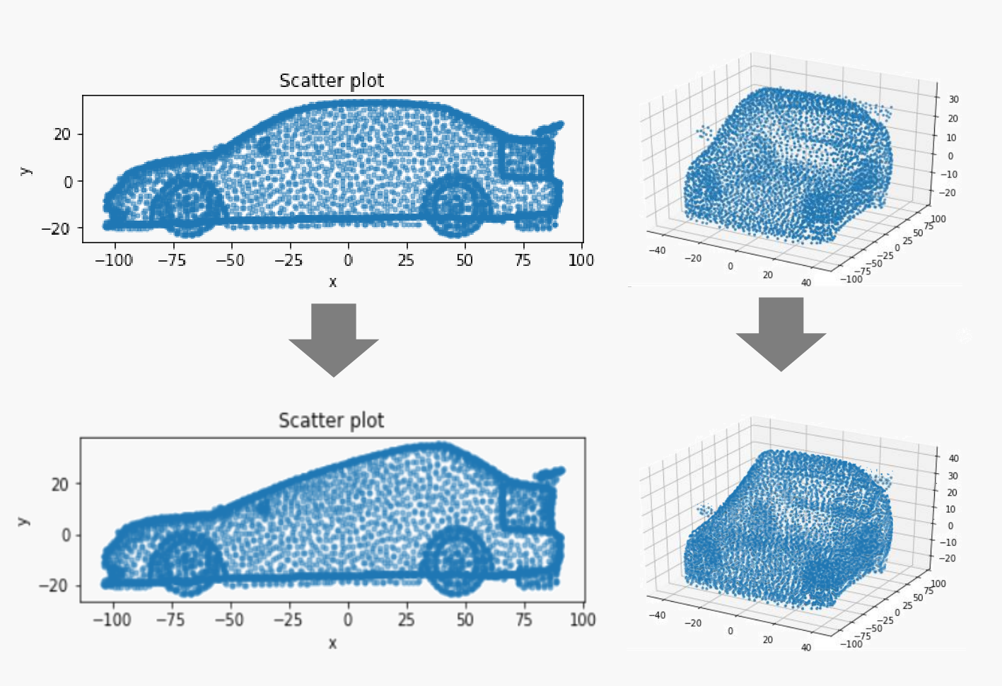
Clinical time series are known for irregular, highly-sporadic and strongly-complex structures, and are consequently difficult to model by traditional state-space models. In this blog, we provide a summary of a recently conducted study [1] on employing variational recurrent neural networks (VRNNs) [2] for forecasting clinical time series, extracted from the electronic health records (EHRs) of patients. Variational recurrent neural networks (VRNNs) combine recurrent neural networks (RNNs) [3] and variational inference (VI) [4], and are state-of-the-art methods to model highly-variable sequential data such as text, speech, time series and multimedia signals in a generative fashion. This study focused on incorporating multiple correlated time series to improve the forecasting of VRNNs. The selection of those correlated time series is based on the similarity of the supplementary medical information e.g., disease diagnostics, ethnicity and age etc., between the patients. The effectiveness of utilizing such supplementary information was measured with root mean square error (RMSE), on clinical benchmark data-set “Medical Information Mart for Intensive Care (MIMIC III)” for multi-step-ahead prediction. In addition, a subjective analysis to highlight the effects of the similarity of the supplementary medical information on individual temporal features e.g., Systolic Blood Pressure (SBP), Heart Rate (HR) etc., of the patients from the same data-set was performed. The results of this research demonstrated that incorporating the correlated time series based on the supplementary medical information can help improving the accuracy of the VRNNs for clinical time series forecasting.
A variational recurrent neural network (VRNN) [2] is the extension of a standard Variational Autoencoder (VAE) [4] to the cases with sequential data. It is a combination of a Recurrent Neural Network (RNN) and a VAE. More specifically, a VRNN employs a VAE at each time-step. However, the prior on the latent variable of this VAE is assumed to be a multivariate Gaussian whose parameters are computed from the previous hidden state of the RNN. The detailed discussion on VRNN and VAE is provided in [2] and [4] respectively. In this study [1], the VRNN is extended in the sense that the multiple correlated temporal signals are also included in the input which improvises the robustness of the model. This is since the model i.e., VRNN, is now forced to learn the additional local patterns of the data space, when conditioned on the additional correlated temporal signals i.e., time series, of the related patients.
An empirical investigation was carried out to quantify the effectiveness of this approach on a clinical benchmark data set “MIMIC III”. However, MIMIC III is a highly complicated data set involving millions of events for approximately 60,000 patients in Intensive Care Units (ICUs). As such, a baseline approach [5] was followed to pre-process the data. After following [5], the resulting pre-processed data set was used to build four models: VRNN, VRNN-I, VRNN-S and VRNN-I-S. The first two models belong to the family of VRNNs whereas the last two models are the extensions of the first two models using this approach. As such, VRNN and VRNN-I act as the baseline models whereas VRNN-S and VRNN-I-S are their improved variations using this approach. All four models are tested for multi-step-ahead predictions with RMSE.
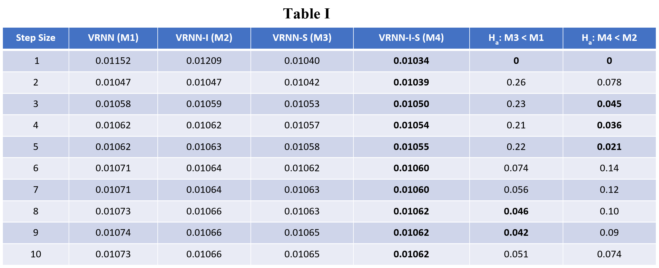
The Average (i.e., for all the temporal variables) RMSE on the test data-set for multi-step-ahead forecasting are presented in Table I. In this table, the first column displays the step size for forecasting. The next four columns present the RMSE with rounded standard deviations using VRNN (M1), VRNN-I (M2), VRNN-S (M3), and VRNN-I-S (M4). The last two columns share the p values resulting from the Mann-Whitney U test. These tests have the alternative hypotheses RMSE (VRNN-S) < RMSE (VRNN) and RMSE (VRNN-I-S) < RMSE (VRNN-I) respectively i.e., these tests find if the improved variations VRNN-S and VRNN-I-S are significantly better than their respective baseline VRNN and VRNN-I. From this table, it can be observed that VRNN-I-S achieves the lowest values of RMSE in all the ten cases. Furthermore, VRNN-S achieves the second lowest error in all the ten cases. From the last two columns in Table I, we find out that in 6/10 cases; at-least one of VRNN-S and VRNN-I-S performs significantly better than the respective baseline as indicated by the p values.
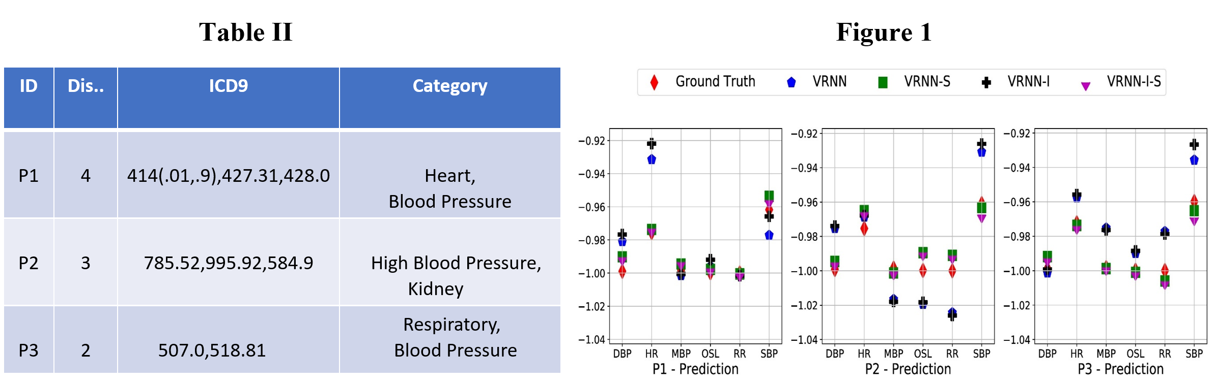
We further perform a simple qualitative analysis to highlight the importance of correlated temporal signals in robust and improved forecasting of VRNNs. We select three patients in the test data-set where VRNN-S and VRNN-I-S both achieve the lowest RMSE. For each of these patients, we select three most similar patients based on disease diagnostics and report the information about the set of common diseases between our selected patients and their corresponding most similar patients in Table II. In this table, the first column shows the identity of each of the three selected patients. The second column reports the number of common diseases between that patient and its three most similar patients. The third column shares the International Classification of Diseases, Ninth Revision (ICD9) codes for the corresponding diseases. The last column categorizes the respective ICD9 codes to the most appropriate disease family (i.e., Heart, Blood Pressure, Kidney, Respiratory) for better interpretation and analysis. After reporting the information about the common diseases, we plot the predictions of all four models on our patients of interest in figure 1. This figure shares the one-step-ahead predicted values (re-scaled) for all six temporal variables for these patients. Considering the first patient (P1) in figure 1; we observe that VRNN-S and VRNN-I-S outperform the baselines on Heart Rate (HR), which is related to the category of the most common diseases for that patient in Table II. Similarly analysing the second patient (P2); we observe that VRNNS and VRNN-I-S outperform the baselines on Systolic Blood Pressure (SBP) which is strongly related to high blood pressure related diseases. Finally, the same analysis is performed for third patient (P3) where VRNN-S and VRNN-I-S achieve superior predictions on Respiratory Rate (RR) and Systolic Blood Pressure (SBP). From figure 1, we verify that incorporating correlated temporal signals indeed helps improving the forecasting accuracy of the VRNNs for clinical time series. This is especially true for the temporal features which are related to the set of the common diseases between the patients.
In this paper, we evaluate the effectiveness of utilizing multiple correlated time series in clinical time series forecasting tasks. Such correlated time series can be extracted from a set of similar patients; where the similarity can be computed on the basis of the supplementary domain information such as disease diagnostics, age and ethnicity etc. As our baselines, we choose VRNN and its variant, which are state-of-the-art deep-generative models for sequential data-sets. From the findings in section V, we believe that the performance of Variational Recurrent models can be improved by including the correlated temporal signals. This is since in 6/10 cases considered in Table I; at-least one of VRNN-S and VRNN-I-S performs significantly better than the baselines as indicated by the p values resulting from the statistical tests. Additionally, it can be observed from figure 1 that the incorporation of multiple correlated time series helps recovering the temporal features related to the common diseases between the patients. On the basis of the points discussed above, it can be argued that discarding such supplementary domain information while analysing clinical data-sets may not be an optimal strategy, since such information may be used to improve the generalization.
[1] Ullah, Sibghat, et al. “Exploring Clinical Time Series Forecasting with Meta-Features in Variational Recurrent Models.” To appear in, 2020 International Joint Conference on Neural Networks (IJCNN).
[2] Chung, Junyoung, et al. “A recurrent latent variable model for sequential data.” Advances in neural information processing systems. 2015.
[3] LeCun, Yann, Yoshua Bengio, and Geoffrey Hinton. “Deep learning.” nature 521.7553 (2015): 436-444.
[4] Kingma, Diederik P., and Max Welling. “Stochastic gradient VB and the variational auto-encoder.” Second International Conference on Learning Representations, ICLR.
[5] Harutyunyan, Hrayr, et al. “Multitask learning and benchmarking with clinical time series data.” Sci Data 6, 96 (2019). https://doi.org/10.1038/s41597-019-0103-9.
The topic of my research is “Multi-criteria Preference Aware Design Optimization”, which is one of the projects of this ECOLE doctoral training program. The main aim of my research is to develop a system which can learn from user experience of designing and support the user by giving multiple suggestions from which the user can choose.
There are several designing frameworks for assisting users like SketchRNN [1], Shadow Draw [2], etc. Regardless of how efficient 2D design tools are, there is a lack of efficient tools for 3D counterparts. But in engineering applications, we mainly need to deal with 3D models for designing. It is more difficult to model a 3D shape of high dimensionality for the complexity of its shape. The design process in the engineering domain is complex, i.e., there are many possible paths leading through the design space and the design space is too large to be navigated by the human designer. So, through my research, we aim to design a system that supports the designer in searching and suggesting for applications in engineering design.
Machine learning and deep learning approaches are the backbones of automated analytical models. But all these approaches are data-driven approaches. So, one of the key aspects of training machine learning models is to gather potential large dataset to train the model. There is existing dataset for 2D sketches [1,2], but for 3D shapes there is no existing dataset to understand the design process.
A key part of my research is to understand the human user-centric design process for engineering applications. Conducting research with human participants in an essential part to understand the human designing process. The most challenging part involves human study as it is time-consuming and difficult with a high number of human participants, which is essential for the system to suggest the multiple options for the designer to choose from. Starting with a simpler idea, we did initial experimental setup to understand human behavior of the design process and categorized them into distinct groups. To overcome the limitations, we propose to use target shape matching optimization whose hyper parameters can be tuned to match human user modification data. For a more detailed explanation, the link below [3] refers.
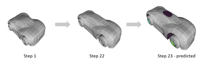
By tuning the hyperparameters of the target shape optimization we can create a digital analogy for human user interactive shape modification. Previous research on sequential modelling approach like Recurrent Neural Networks (RNNs) has been used to model sequences from 2D design tasks, such as human drawing [2]. So, we further experimented on using RNNs to learn the past changes gathered from optimizations data and predict the next possible steps in engineering design application. Below is an example from our model predictions of next possible change in the design (Figure 1).
We only include a basic idea of a design assistance system and why it is necessary for engineering applications and then verified our initial approach to come up with a suitable model. I will keep you informed about our work in my future blog.
[1] Y. J. Lee, C. L. Zitnick, and M. F. Cohen, “ShadowDraw: real-time user guidance for freehand drawing,” 2011.
[2] D. Ha and D. Eck, “A neural representation of sketch drawings,” in 6th International Conference on Learning Representations, ICLR 2018, Vancouver, BC, Canada, April 30 – May 3, 2018, Conference Track Proceedings, 2018.
[3] Saha, S., Rios, T.., Minku, L.L., Yao, X., Xu, Z., Sendhoff, B., “Optimal Evolutionary Optimization Hyper-parameters to Mimic Human User Behavior,” 2019 IEEE Symposium Series on Computational Intelligence (SSCI), Xiamen, China, 2019, pp. 858-866
[4] S. Saha., Rios, T.D., Sendhoff, B., Menzel, S., Bäck, T., Yao, X., Xu, Z., & Wollstadt, P., “Learning Time-Series Data of Industrial Design Optimization using Recurrent Neural Networks,” 2019 International Conference on Data Mining Workshops (ICDMW), Beijing, China, 2019, pp. 785-792.
During the PhD we are constantly challenged to find solutions for technical problems and push the knowledge frontier in our fields a little further ahead. As a measure to support controlling the current COVID-19 epidemic, many of us started working in home office a couple of weeks ago and, therefore, we face new sorts of problems, such as staying healthy, connected and focused on our work [1,2]. Hence, we wrote down a few pros and cons of working from home in our notepads, as well as some tips to “survive” the home office season, which we are sharing with you in this post.
Working from home can be very pleasant and fruitful. Apart from tasks that require special hardware, for example, running chemistry experiments in a lab, we usually can do a lot with a notebook, access to the internet and remote access to our workstation in the office. Furthermore:
Working at home can be very convenient, however, it has some drawbacks, especially in the long term. In such cases, it’s common to feel isolated and less productive [1], because:
Staying healthy is now the priority, so going back to the office is not yet an option, so all we can do is focus on improving our home-office experience by minimizing the cons in our list. Here is a short list of tips we came up with for tackling the drawbacks of working during the quarantine:
Finally, we hope our impressions and tips help you to go through this exceptional working conditions. It is not ideal for many of us, but it is temporary and very important to contain the epidemic. Let’s do our part and help keeping our communities safe.
[1] B. Lufkin, “Coronavirus: How to work from home, the right way”, bbc.com, 2020. [Online]. Available: https://www.bbc.com/worklife/article/20200312-coronavirus-covid-19-update-work-from-home-in-a-pandemic. [Accessed: 30- Mar- 2020].
[2] S. Philipp and J. Bexten, “Home Office: Das sind die wichtigsten Vor- und Nachteile – ingenieur.de”, ingenieur.de – Jobbörse und Nachrichtenportal für Ingenieure, 2020. [Online]. Available: https://www.ingenieur.de/karriere/arbeitsleben/alltag/home-office-das-wichtigsten-vorteile-nachteile/. [Accessed: 30- Mar- 2020].
It has been during my Master’s thesis internship when I first heard about the Early Stage Researcher (ESR) figure. PhD student and industry researcher at the same time, I thought it was the perfect mix for my future development. Thus, after been graduated, I started looking for a job and finally, I found the one I was interested in: Machine Learning ESR. I applied for this position, did the interview and got hired… The beginning of a new phase of my life, within the ECOLE project.
Nowadays, we are living in the digital era and the amount of user-generated data is exponentially growing every day. In this context, users usually explain what they like, dislike or think in the form of textual comments (e.g. tweets, social media posts, reviews). Leveraging the rich latent information contained in the user-generated data available can be crucial for many purposes. For example, an automobile company can launch a face-lift car that would satisfy customers more than before, by mining history order and users’ feedback [1]. Recently, research in the manufacturing industry focuses on developing advanced text mining approaches to discover hidden patterns, to predict market trends and to learn customer preferences and unknown relations, for improving their competitiveness and productivity. Keeping this in mind, my objective within ECOLE is on developing statistical machine learning and probabilistic models for preference learning. The focus will be not only on obtaining good results but also on getting interpretability of the outputs and on providing a measure of confidence about them. ECOLE aims at solving a series of related optimisation problems, instead of treating each problem instance in isolation, thus the learned information could be integrated to include preference constraints in multi-criteria optimization frameworks (e.g. product design, where structural, aerodynamics and aesthetic constraints have to be considered simultaneously).
Now, it has been more than a year since I have been involved in ECOLE. During this period, I had the possibility to know and to work with the other ESRs, to learn a lot from the experienced supervisors (from academia and industry), and to travel and visit several countries for attending summer schools, workshops, conferences. The mixture of different cultures, backgrounds and the collaboration between academia and industry has created an inspiring and motivating environment to improve either soft-skills, technical skills and grow as a researcher.

[1] Ray Y Zhong, Xun Xu, Eberhard Klotz, and Stephen T Newman. Intelligent manufacturing in the context of industry 4.0: a review. Engineering, 3(5):616–630, 2017.
Dynamic multi-objective optimization problems (DMOPs) involve multiple conflicting and time-varying objectives, which widely exist in real-world problems. Evolutionary algorithms are broadly applied to solve DMOPs due to their competent ability in handling highly complex and non-linear problems and most importantly solving those problems that cannot be addressed by traditional optimization methods.
Without generality, the minimization problem is considered here and a DMOP [1] can be mathematically formulated as follows:
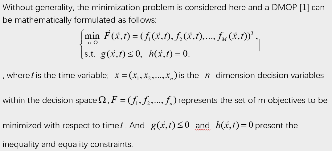
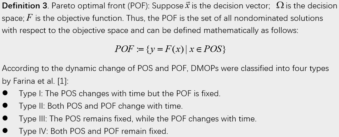
Evolutionary algorithms for solving DMOPs are called dynamic multi-objective evolutionary algorithms (DMOEAs) [2]. In the development of DMO, a mature framework of DMOEAs [3] has been proposed by researchers, as shown in Fig. 1.
Fig. 1. Flowchart of DMOEAs
The detailed steps of the framework of DMOEAs are as follows:
Most existing work in DMO mainly focus on how to improve the effectiveness of response mechanisms.
[1]. M. Farina, K. Deb, P. Amato, Dynamic multiobjective optimization problems: test cases, approximations, and applications, IEEE Trans. Evolut. Comput. 8 (5) (2004) 425–442.
[2]. S. Yang and X. Yao, Evolutionary Computation for Dynamic Optimization Problems. Springer, 2013, vol. 490.
[3]. G. Ruan, G. Yu, J. Zheng, J. Zou, and S. Yang, “The effect of diversity maintenance on prediction in dynamic multi-objective optimization,” Applied Soft Computing, vol. 58, pp. 631–647, 2017.
Time flies fast. It has been almost over one year since I joined ECOLE. And it has been an exciting year. Travelling between Birmingham, Warsaw, Leiden, Berlin, Coimbra and Xiamen. Listening to talks in state of the art on research in Evolutionary Computation and Machine Learning. Attending workshops in the research institutions of two world-known tech companies. The opportunities promised and given by the Innovative Training Network have not fallen short. But aside from all the excitement and activities, who am I, what do I do and what is that drove me to ECOLE in the first place?
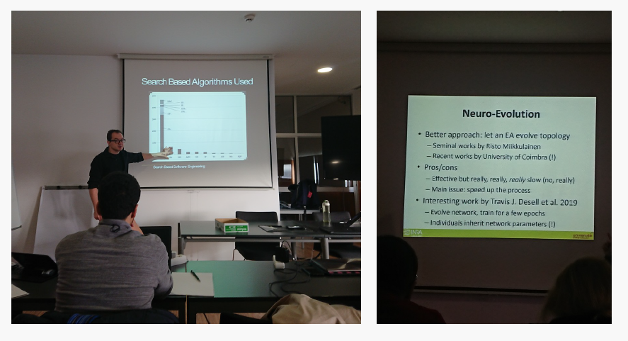
Well, my prior academic pursuits were in Theoretical Nuclear Physics at the Technical University Darmstadt. And while I of course enjoyed studying the field and gaining understanding into the inner subnuclear workings of the world, I felt at times the research self was missing out in some way on my initial fascinations which took me too it. So, where to go else? Stumbling upon ECOLE was to be honest a bit of a lucky coincidence. I was working prior at software company while looking for PhD and residency programs, when a friend of mine was recommending me the posting for an Early Stage Researcher position he found at one of the partner institutions. I applied, was interviewed and subsequentially have been offered the position. It has been a bit unusual for me to travel this much for the Marie Curie Fellowship, but I am happy to have found a new home. And with Computational Intelligence research being situated at the intersection between Natural Computation and Artificial Intelligence, there is still plenty of space for me to philosophize about nature, while keeping in touch with reality through real-world problems.

ECOLE is especially great in regards of opportunities to learn, grow and try out new things. I particularly had a lot of fun (but also stress) with preparing and giving a short keynote-style public talk on nature-inspired artificial intelligence for the popular science segment of the Z2X festival in Berlin last August. The talk was luckily to be held lightweight and in front of a small audience. I decided to talk about the history and inspirations behind current popular methods and highlight evolutionary approaches as a means for creative problem-solving. While part of the audience seemed to have got lost with some of the bare technicalities, the main ideas sticked. Which was the most important thing for me. I was thus more than happy to have received and interesting questions in return. By the way: I am planning to put my practice slides online soon, if you are interested, feel free to take a look. The actual talk was given completely in oral form, as I was informed one day prior that the beamer was missing, but it worked out.
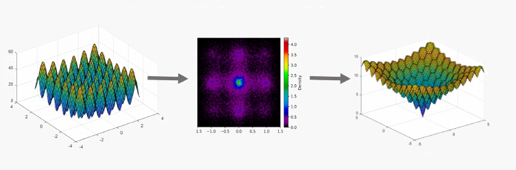
So, what’s up for the future? Currently, I work on model-based approaches as a means to tackle the transfer learning problem in continuous optimisation. A bit of a complicated idea, but I find this notion to be intuive and interesting to explore. In any way, I will keep you updated about my work in a future blog post. Until then, everyone keep up with the good work! 🙂


The adaptive synthetic (ADASYN) sampling technique is a method that aims to adaptively generate minority samples according to their distributions [5]. The main improvement compared to SMOTE is the samples which are harder to learn are given higher importance and will be oversampled more often in ADASYN. The general idea of ADASYN is shown in Figure 3.

[1]. He, H. and Garcia, E.A., 2009. Learning from imbalanced data. IEEE Transactions on knowledge and data engineering, 21(9), pp.1263-1284
[2]. Ganganwar, V., 2012. An overview of classification algorithms for imbalanced datasets. International Journal of Emerging Technology and Advanced Engineering, 2(4), pp.42-47.
[3]. Santos, M.S., Soares, J.P., Abreu, P.H., Araujo, H. and Santos, J., 2018. Cross-validation for imbalanced datasets: Avoiding overoptimistic and overfitting approaches [research frontier]. ieee ComputatioNal iNtelligeNCe magaziNe, 13(4), pp.59-76.
[4]. Chawla, N.V., Bowyer, K.W., Hall, L.O. and Kegelmeyer, W.P., 2002. SMOTE: synthetic minority over-sampling technique. Journal of artificial intelligence research, 16, pp.321-357.
[5]. He, H., Bai, Y., Garcia, E.A. and Li, S., 2008, June. ADASYN: Adaptive synthetic sampling approach for imbalanced learning. In 2008 IEEE International Joint Conference on Neural Networks (IEEE World Congress on Computational Intelligence) (pp. 1322-1328). IEEE.


[1] Lütkepohl, Helmut. New introduction to multiple time series analysis. Springer Science & Business Media, 2005.
[2] LeCun, Yann, Yoshua Bengio, and Geoffrey Hinton. “Deep learning.” nature 521.7553 (2015): 436-444.
[3] Williams, Ronald J., and David Zipser. “A learning algorithm for continually running fully recurrent neural networks.” Neural computation 1.2 (1989): 270-280.
[4] Rangapuram, Syama Sundar, et al. “Deep state space models for time series forecasting.” Advances in Neural Information Processing Systems. 2018.
[5] Qiu, Jinwen, S. Rao Jammalamadaka, and Ning Ning. “Multivariate Bayesian Structural Time Series Model.” Journal of Machine Learning Research 19.68 (2018): 1-33.
[6] Harutyunyan, Hrayr, et al. “Multitask learning and benchmarking with clinical time series data.” arXiv preprint arXiv:1703.07771 (2017).
[7] Guo, Tian, et al. “Robust online time series prediction with recurrent neural networks.” 2016 IEEE International Conference on Data Science and Advanced Analytics (DSAA). Ieee, 2016.
Innovative Training Networks (ITN) drive scientific excellence and innovation. They bring together universities, research institutes and other sectors from across the world to train researchers to doctorate level.

Sharing technical concepts, experience, applications in industry.